Gradient Based Motion Estimation

Revision as of 22:44, 23 April 2006

Detecting sub-pixel shifts

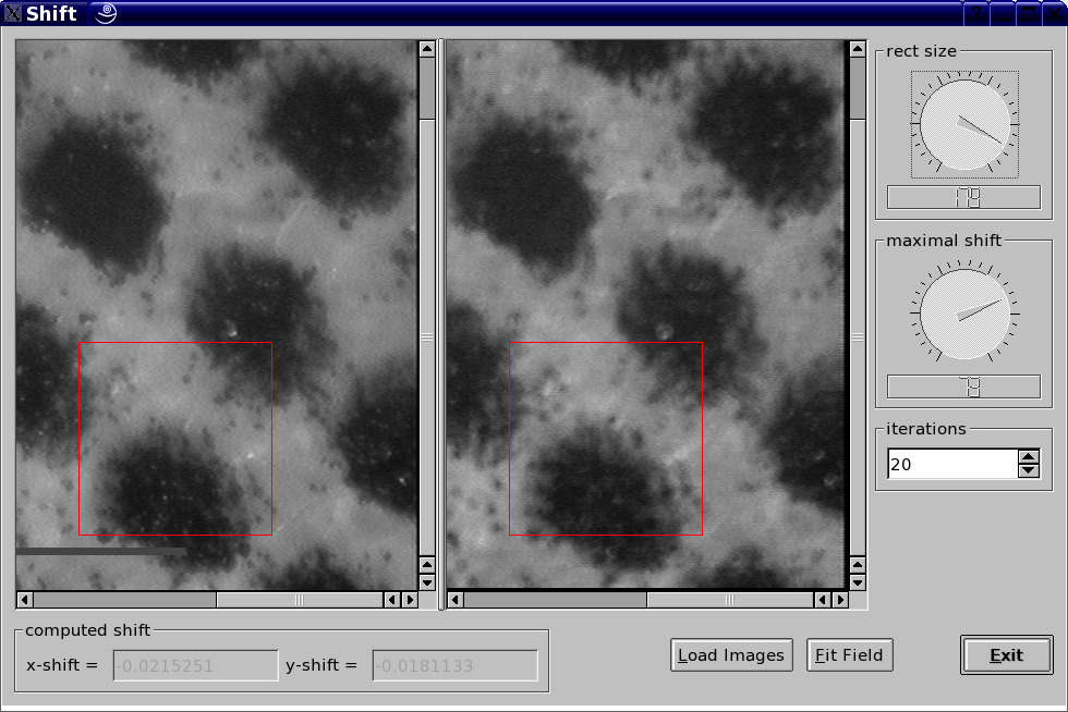
Using gradient based motion estimation is good at detecting sub-pixel shifts. During an investigation on depth of defocus, this software was developed for compensating the misalignment of a focus-drive.

The local gradient <math>\cfrac{\delta g}{\delta\vec{x}}</math> of the gray values and the gradient in time <math>\cfrac{\delta g}{\delta t}</math> are related to each other in the first order:

<math>\Big(\cfrac{\delta g}{\delta x_1}(\vec{x},t)\ \cfrac{\delta g}{\delta x_2}(\vec{x},t)\Big)^\top\cdot\vec{v}(\vec{x},t)\approx-\cfrac{\delta g}{\delta t}(\vec{x},t)</math> where <math>g\in\mathbb{R}^2\times\mathbb{R}\mapsto\mathbb{R}</math> is a video and <math>\vec{v}\in\mathbb{R}^2\mapsto\mathbb{R}^2</math> a motion vector field.

Using the model <math>\vec{v}\big(\begin{pmatrix}x_1\\x_2\end{pmatrix}\big)=\begin{pmatrix}a_1+b_1\,x_1\\a_2+b_2\,x_2\end{pmatrix}</math> this becomes a least square problem: <math>\begin{pmatrix} \cfrac{\delta g}{\delta x_1}(\vec{p_1}) & p_{1,1}\,\cfrac{\delta g}{\delta x_1}(\vec{p_1}) & \cfrac{\delta g}{\delta x_2}(\vec{p_1}) & p_{1,2}\,\cfrac{\delta g}{\delta x_2}(\vec{p_1}) \\ \vdots & \vdots & \vdots & \vdots\\ \cfrac{\delta g}{\delta x_1}(\vec{p_n}) & p_{n,1}\,\cfrac{\delta g}{\delta x_1}(\vec{p_n}) & \cfrac{\delta g}{\delta x_2}(\vec{p_n}) & p_{n,2}\,\cfrac{\delta g}{\delta x_2}(\vec{p_n}) \\ \end{pmatrix} \begin{pmatrix} a_1\\b_1\\a_2\\b_2 \end{pmatrix}= \begin{pmatrix} -\cfrac{\delta g}{\delta t}(\vec{p_1})\\\vdots\\ -\cfrac{\delta g}{\delta t}(\vec{p_n}) \end{pmatrix} +\vec{\epsilon} </math> where <math>a_1</math>, <math>a_2</math> are denoting the shift and <math>b_1</math>, <math>b_2</math> are denoting the scale between the two images.

The result can be improved by applying the least square algorithm iteratively to the compensated images. It may also be necessary to apply a low-pass filter to the images before performing motion estimation.