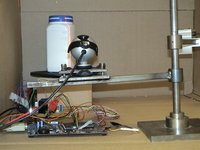
Mimas Camera Calibration
From MMVLWiki
 |
 |
 |
| Table of contents |
Calibration
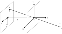
Plane-to-camera homography
Let 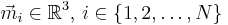 be the homogeneous coordinate (http://en.wikipedia.org/wiki/Homogeneous_coordinates#Use_in_computer_graphics) of the ith point on the planar calibration-object and let
  be the homogeneous coordinate of the corresponding pixel in the camera-image. Further let
  be an equivalence relation (http://en.wikipedia.org/wiki/Equivalence_relation) defined by

If the camera-system does an ideal central projection (e.g. no distortion), the projective transformation (the Homography (http://en.wikipedia.org/wiki/Homography)) can be modelled using  as follows
or more elaborately
 where
where  is the zero-mean error-vector in the observation of the ith point in the camera-image.
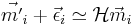
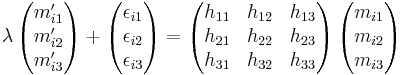
Using 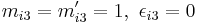 and
and 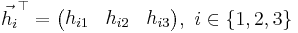 the
model can be reformulated to
the
model can be reformulated to
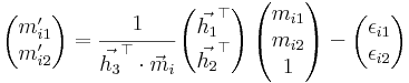 or
or 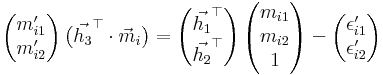 with
with
![\vec{\epsilon^\prime}_i=\big[\vec{h_3}^\top\cdot\vec{m}_i\big]\,\vec{\epsilon}_i](math_3b4d.png) and using
and using 
It is assumed, that the vectors  have equal variances (i.e.
 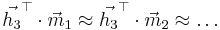 ) so that the Gauss-Markov theorem (http://en.wikipedia.org/wiki/Gauss-Markov_theorem) can be applied using
  as error-vectors. In this case the miminum least-squares estimator (http://en.wikipedia.org/wiki/Least_squares) is the best linear estimator.
Each point-pair yields the following system of two linear equations

Isolating the elements of the unknown matrix  gives
gives
The combined system of all linear equations is
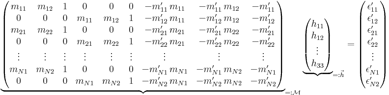
To avoid the trivial solution  the constraint
  is introduced without loss of generality.
The calibration problem now has been reduced to the problem of finding  such that
-
 is minimal and
-

 can be computed using the Singular value decomposition (http://en.wikipedia.org/wiki/Singular_value_decomposition)
  , because these are the properties of the right handed singular vector
  with the smallest singular value σ1 (where
  ). I.e.
  .
.
Knowing the homography already is sufficient for the Interactive Camera-Projector System.
Intrinsic and extrinsic camera parameters
Please see references below ...
See Also
- Mimas
- Bright : A project using the camera calibration to build a laser-line based 3-D scanner.
- Interactive Camera-Projector System
External Links
- Julien Faucher's report (http://vision.eng.shu.ac.uk/manuel/bright/report_faucher.pdf)
- Zhengyou Zhang: A Flexible New Technique for Camera Calibration (http://research.microsoft.com/%7Ezhang/Calib/)
- Ballard and Brown: Computer vision (chapter A1.8.1 on camera calibration) (http://homepages.inf.ed.ac.uk/rbf/BOOKS/BANDB/bandb.htm)
- Augmented Reality with Sony Playstation (google video) (http://video.google.co.uk/videoplay?docid=-6642378035529869995#9m43s)
- Camera calibration toolbox for Matlab (http://www.vision.caltech.edu/bouguetj/calib_doc/)
- GML Camera Calibration toolbox (http://research.graphicon.ru/calibration/gml-c-camera-calibration-toolbox.html)
- EPFL camera calibration software (http://cvlab.epfl.ch/software/bazar/calib.php)
- MRPT camera calibration software (http://www.youtube.com/watch?v=BkZkq6zPwQM&feature=player_embedded#!)
- OpenCV / WillowGarage camera calibration (http://opencv.willowgarage.com/documentation/python/camera_calibration_and_3d_reconstruction.html)
![]()

